In the previous article we created a tileable noise texture with different noise textures in each channel.

In this article we combine the layers to create scrolling 2D clouds. Like this.
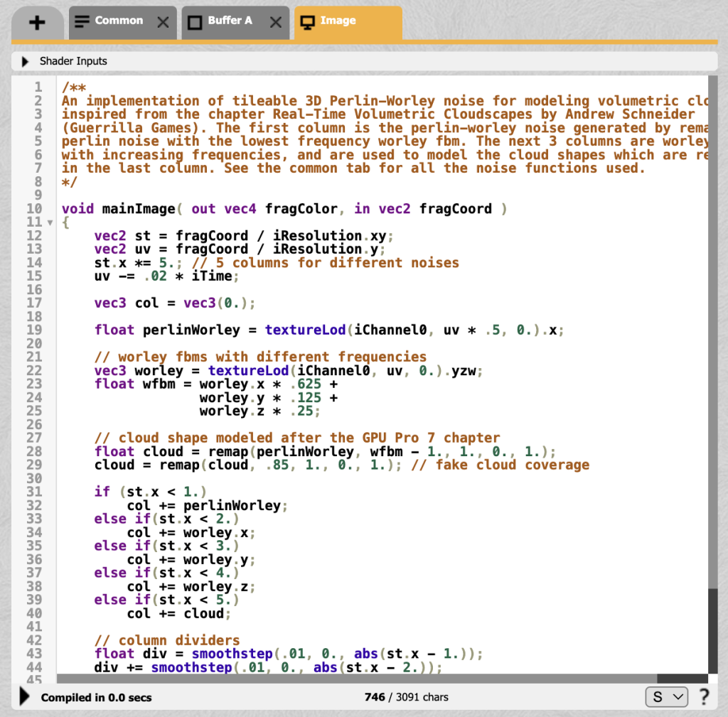
As previously mentioned we’re refactoring this ShaderToy example. The code uses a common library which we created and a pre-rendered tileable texture. The final step is shown in the screengrab below.

This code creates 5 columns. We’re only interested in the 5th column where the layers are combined to create a single layer of billowy clouds. We will need to create the updated uv value based on time and reproduce the cloud value.
We create a uv variable, uv1, that is the interpolated uv value minus the current time in seconds multiplied by 0.02. Then we take the fractional part of this, that is 1.23 becomes 0.23. Now we have a uv value we sample the storageTexture, the pre-calculated tileable multi-layered noise. Then we extract the red channel as perlinWorley and the remaining channels as worley. We combine the three worley layers at a variety of strengths, wfbm. Then we remap the perlinWorley variable using wfbm minus a uniform, wfbmctrl, which is initially set to 1 as the lower end of the source range to 1 as the high value of the source range, mapped to [0-1]. Then we increase the cropping by remapping the remapped value from the range [uniform, pwctrl-1] to [0-1]. I’ve added a gui to let you experiment with these values which should help you understand their effect.
const wfbmctrl = uniform( float( 1. ) );
const pwctrl = uniform( float( 0.85 ) );

const fragmentTSL = Fn(({ storageTexture }) => {
  const uv1 = vec2(uv()).sub(time.mul(0.02)).toVar();
  uv1.assign( fract( uv1 ) );

  const texel = texture(storageTexture, uv1, 0).toVar();

  const perlinWorley = texel.r.toVar();
  const worley = texel.gba.toVar();

  // worley fbms with different frequencies
  const wfbm = worley.r
      .mul(0.625)
      .add(worley.g.mul(0.125))
      .add(worley.b.mul(0.25))
      .toVar();

  // cloud shape modelled after the GPU Pro 7 chapter
  const cloud = remap(perlinWorley, wfbm.sub(wfbmctrl), 1, 0, 1).toVar();
  cloud.assign(saturate(remap(cloud, pwctrl, 1, 0, 1))); // fake cloud coverage

  return vec4(1, 1, 1, cloud);
});

material.fragmentNode = fragmentTSL({ storageTexture });
The final colour value is set to white with the calculated cloud value used as the alpha value.
Now we have 2D clouds it’s time to move into the third dimension. We’ll begin to do that in the next installment.
If you find these articles useful, perhaps you can buy me a coffee by clicking the button below. It might encourage me to write more.
Signup to my mailing list.
